If a leaf were to fall into the river it would be swept along a path determined by those currents. Using a direction field, we can see many possibile solutions. Differential Equations with Events » WhenEvent — actions to be taken whenever an event occurs in a differential equation. Solve a differential equation representing a predator/prey model using both ode23 and ode45. thickness = 1, orientation = [-40,80], title=`Lorenz Chaotic Attractor`); Plotting solutions to differential equations, © Maplesoft, a division of Waterloo Maple
odephas3 Three-dimensional phase plane plots. As mentioned, the differential equation reflects the fact that the value of the derivative of a solution at time is given by . Solutions to Simple Differential Equaions. E.g., for the differential equation y'(t) = t y 2 define. and plot M1 against T1. Even though the situation is a bit more complicated, the method still works just as well. The following steps show a simple example of using dsolve() to create a differential solution and then plot it: Type Solution = dsolve(‘Dy=(t^2*y)/y’, ‘y(2)=1′, ‘t’) and press Enter. The problems above had simple answers because each differential equation could be integrated to get a solution. Activity. Differential Equations with Events » WhenEvent â actions to be taken whenever an event occurs in a differential equation. As an example, take the equation with the initial conditions and : 1.096000 Median ⦠plotting differential-equations A time series plot for a solution to (??) Please forgive me if I'm setting you off on a wild goose chase; it's been over 50 years since I had DE. color = blue, linecolour=red,arrows=MEDIUM ); Here is an example where the differential equation is very sensitive to the initial point chosen. The default identifier is y1. MATLAB Tutorial on ordinary differential equation solver (Example 12-1) Solve the following differential equation for co-current heat exchange case and plot X, Xe, T, Ta, and -rA down the length of the reactor (Refer LEP 12-1, Elements of chemical reaction engineering, 5th edition) Slope field for y' = y*sin(x+y) Activity. we are going to solve the Ordinary Differential Equation dy/dt=exp(-t) … In order to access the routines in the DEtools package by their short names, the with command has been used. 1 â® Vote. You will see a black border appear around the graph. Example 3: Solving Nonhomogeneous Equations using Parameterized Functions . 2 minute read. POWERED BY THE WOLFRAM LANGUAGE. Your line graph will plot the points on an x-y axis to allow you to identify the point where your simultaneous differential equations meet. To plot the numerical solution of an initial value problem: For the initial condition y(t0)=y0 you can plot the solution for t going from t0 to t1 using ode45(f,[t0,t1],y0). Calculus, Differential Equation A direction field (or slope field / vector field) is a picture of the general solution to a first order differential equation with the form Edit … Type the differential equation, y1 = 0.2 x2. Get help with your Differential equation homework. Differential equation ÄVLPLODUWRIRUPXODRQSDSHU. Differential equation or system of equations, specified as a symbolic equation or a vector of symbolic equations. DEplot( deq, y(x), x=-2..2, [[ y(0) = 0 ]], y=-8..8, linecolour=red, color = blue, stepsize=.1,arrows=MEDIUM ); The curve in red is the solution which follows the flow of the direction field and passes through (0,0). DEplot( deq, y(x), x=-3..3, [[ y(0)= k/4 ] $ k = -11..11], y=-3..3,
X represents L and Y represents theta. Additional information is provided on using APM Python for parameter estimation with dynamic models and scale-up to large-scale problems. These two methods are based on interpreting the derivative alternatively as either the slope of a tangent line or as the velocity of a particle. Plotting Two-Dimensional Differential Equations. Differential equation. color = blue, linecolour=red, arrows=MEDIUM ); >
f is the right hand side of the differential equation; a function, external, string or list. >
To embed this widget in a post, install the Wolfram|Alpha Widget Shortcode Plugin and copy and paste the shortcode above into the HTML source. Juan Carlos Ponce Campuzano. color = aquamarine,linecolour=sin(t*Pi) ); Unlike a textbook, you are not limited to simply looking at his graph. Calculus - Slope Field (Direction Fields) Activity. Introduction to Python. color = blue, linecolour=red, arrows=MEDIUM ); Here is another family generated by choosing different y intercepts. This shows a relationship between the second derivative of y with respect to x … The Wolfram Language can find solutions to ordinary, partial and delay differential equations (ODEs, PDEs and DDEs). Here is a brief summary of the settings: Solution Method: You have a choice of using Euler or Runge-Kutta as the numerical solution method. There are two different methods for visualizing the result of numerical integration of differential equations of the form (?? odeprint Print to command window. Solving Partial Differential Equations. Erik Jacobsen. 1. Free Vibrations with Damping. Inc. 2019. k = velocity of growth = 1/s. Initial conditions are also supported. One typical use would be to produce a plot of the solution. dy dx + xey 4 for 1
Visualizing differential equations in Python. I've got the following differential equation: dN (t)/dt - ( (k - (a*N (t)))*N (t)) = f (t) This is the logistic law of population growth. In the equation, represent differentiation by using diff. Graphing Differential Equations. I want to solve this equation in such a way to get the value of theta from the 1st equation and use this value in the second equation. Ken Schwartz. The van 't Hoff equation relates the change in the equilibrium constant, K eq, of a chemical reaction to the change in temperature, T, given the standard enthalpy change, ΔH ⊖, for the process.It was proposed by Dutch chemist Jacobus Henricus van 't Hoff in 1884 in his book Études de dynamique chimique (Studies in Dynamic Chemistry). If eqn is a symbolic expression (without the right side), the solver assumes that the right side is 0, and solves the equation eqn == 0.. It returns solutions in a form that can be readily used in many different ways. This is a differential equation. DEplot3d(deq, {x(t),y(t),z(t)}, t=0..100, [[x(0) = 10, y(0)= 10,z(0)= 10]],
Hill plot. C. Plotting Solutions to Parametric Differential Equations _____ We can also plot solutions to parametric differential equations > deq := [ diff(x(t),t)= 4 - y(t),diff(y(t),t)= x(t) - 4 ]; > DEplot( deq, [x(t),y(t)],t= 0..25, [[x(0)=0,y(0)=0]], stepsize=.05, arrows = medium, color = coral,linecolor= 1 + .5*sin(t*Pi/2), method=classical[foreuler]); Calculus: Integral with adjustable bounds. Activity. $laplace\:y^'+2y=12\sin\left (2t\right),y\left (0\right)=5$. A solution to a differential equation is a function that satisfies the differential equation. This agrees with our plot. dy represents first order derivative dy/dt. There are many methods to solve differential equations â such as separation of variables, variation of parameters, or my favorite: guessing a solution. Step 1 Enter "X" into cell A1 of your Excel worksheet (without quotes here and throughout). Equations Speeding up Outline I How to specify a model I An overview of solver functions I Plotting, scenario comparison, I Forcing functions and events I Partial di erential equations with ReacTran I … You can study linear and non-linear differential equations and systems of ordinary differential equations (ODEs), including logistic models and Lotka-Volterra equations (predator-prey models). Each point will specify a different solution. arrows = medium, color = coral,linecolor= 1 + .5*sin(t*Pi/2),
For example say, x1(dot) = -x2 + (x1)^2 -(x1*x2) x2(dot) = x1 + (x1*x2) Thanks in advance! Differential Equation Calculator. DEplot( deq, [x(t),y(t)],t= 0..25, [[x(0)=0,y(0)=0]], stepsize=.05,
color = blue, linecolour=green, arrows=MEDIUM ); C. Plotting Solutions to Parametric Differential Equations, We can also plot solutions to parametric differential equations. Thus the slope will look like. A solution to a differential equation is a function that satisfies the differential equation. The integrated equations produce results that are pure imaginary. In this section we will do the same thing - plot a direction field and various solutions which flow as trajectories in the direction field. k = velocity of growth = 1/s. Thus this is what we want to plot. ODE entry line: ⢠y1 ODE identifier ⢠Expression ⦠stepsize=.02, x = -20..20, y=-25..25,z= 0..50, linecolour=sin(t*Pi/3),
[[x(0)=1,y(0)=.6 ]], stepsize=.05,arrows = small,
Stream plots for a single equation. You can switch back to the summary page for this application by clicking here. i am new in Mathematica please help me. Differential equations can be divided into several types. Differential equation solution: Step-by-step solution; Plots of sample individual solutions: Sample solution family: Possible Lagrangian: Download Page. Solve a system of several ordinary differential equations in several variables by using the dsolve function, with or without initial conditions. One of the first and most famous example of a chaotic attractor is the Lorenz Attractor defined by three parametric differential equations. Differential Equations. Since this is a simple differential equation, obviously the solutions are all of the form x3 - x + C. In order to graph a solution we need to pick a point that the curve passes through. $$\frac{dy(t)}{dt} = -k \; y(t)$$ The Python code first imports the needed Numpy, Scipy, and Matplotlib packages. Example: To plot the solution of ⦠>
A second order ordinary differential equation is given below 20x"+cX+20x=20 For C = 10, 40, and 300 plot y versus t from t =0 to 30 on the same graph. Odd choice, but that's okay! NeumannValue â specify Neumann and Robin conditions The arguments to dsolve() consist of the equation you want to solve, the starting point for y (a condition), and the name of the independent variable. The set of all of these solutions form a family of solutions. I think in this case it would help for you to solve the differential equation for y. Edit Seems my math is wrong per other answer! $y'+\frac {4} {x}y=x^3y^2$. In this project we will use the following command packages. Differential Equations A first-order ordinary differential equation (ODE) can be written in the form dy dt = f(t, y) where t is the independent variable and y is a function of t. A solution to such an equation is a function y = g(t) such that dgf dt = f(t, g), and the solution will ⦠How to plot a differential equation?. You can use this to plot solutions. The calculator will find the solution of the given ODE: first-order, second-order, nth-order, separable, linear, exact, Bernoulli, homogeneous, or inhomogeneous. In this post, we try to visualize a couple simple differential equations and their solutions with a few lines of Python code. Consider the example. Differential equation,general DE solver, 2nd order DE,1st order DE. color = blue, linecolour=red, arrows=MEDIUM ); B. A tiny change in the starting point of a tragectory can lead to very large differences as the object travels pathes following the direction feild. Equations Partial Di . diff(y(t),t) = y(t)*(1 - 4*x(t) - 3*y(t)) ]; >
The following steps show a simple example of using dsolve() to create a differential solution and then plot it: Type Solution = dsolve(âDy=(t^2*y)/yâ, ây(2)=1â², âtâ) and press Enter. share | improve this question | follow | edited Jul 5 '19 at 15:50. As an example, take the equation with the initial conditions and : The DEplot routine from the DEtools package is used to generate plots that are defined by differential equations. dN(t)/dt = the derivative of N(t) = change of # individuals = #individuals/s. Simple Harmonic Motion. laplace y′ + 2y = 12sin ( 2t),y ( 0) = 5. Python Libraries. Commented: Star Strider on 24 Mar 2015 Accepted Answer: Star Strider. f(t) = production function = #individual/s. Plotting system of differential equations. Use Matlab to solve the following differential equation and plot the solution. You may reference the identifier in the entry line. Solve a System of Differential Equations. Below are examples that show how to solve differential equations with (1) GEKKO Python, (2) Euler's method, (3) the ODEINT function from Scipy.Integrate. The equation is written as a system of two first-order ordinary differential equations (ODEs). Setup. These functions are for the numerical solution of ordinary differential equations using variable step size Runge-Kutta integration methods. One typical use would be to produce a plot of the solution. Juan Carlos Ponce Campuzano. Now we have a differential equation that is a bit more complicated. equation is given in closed form, has a detailed description. .). For example, the following script file solves the differential equation y = ry and plots the solution over the range 0 ⤠t ⤠0.5 for the case where r = -10 and the initial condition is y(0) = 2. odephas2 Two-dimensional phase plane plots. DEplot( deq ,y(x), x=-3..3, [[ y(0)=0 ]],
To embed this widget in a post on your WordPress blog, copy and paste the shortcode below into the HTML source: To add a widget to a MediaWiki site, the wiki must have the. NDSolve solves a differential equation numerically. DSolveValue takes a differential equation and returns the general solution: (C[1] stands for a constant of integration.) The curve that the leaf sweeps out corresponds to a solution of the differential equation. Numerically solving a linear system to obtain the solution of the beam-bending system represented by the 4 t h-order differential equation in R First create a near-tri-diagonal matrix A that looks like the following one, it takes care of the differential coefficients of the beam equation along with all the boundary value conditions. This makes DifferentialEquations.jl a full-stop solution for differential equation analysis which also achieves high performance. These equations are evaluated for different values of the parameter μ.For faster integration, you should choose an appropriate solver based on the value of μ.. For μ = 1, any of the MATLAB ODE solvers can solve the van der Pol equation efficiently.The ode45 solver is one such example. deq := [diff(x(t),t) = x(t)*1(1 - 1*x(t) - 4*y(t)),
y=-8..8, color = blue, stepsize=.05, linecolour=red, arrows=MEDIUM ); >
>
In other words, the slope of the tangent line to the solution is known and is given by the right hand side of the differential equation. Type and execute this line before begining the project below. Basics of Python. Get the free "General Differential Equation Solver" widget for your website, blog, Wordpress, Blogger, or iGoogle. Introduction Model Speci cation Solvers Plotting Forcings + EventsDelay Di . Partial Differential Equations » DirichletCondition â specify Dirichlet conditions for partial differential equations. Below is an example of solving a first-order decay with the APM solver in Python. Vote. Quick Start 8-3 Quick Start 1 Write the ordinary differential equation as a system of first-order equations by making the substitutions Then is a system of n first-order ODEs. This example shows you how to convert a second-order differential equation into a system of differential equations that can be solved using the numerical solver ode45 of MATLAB®.. A typical approach to solving higher-order ordinary differential equations is to convert them to systems of first-order differential equations, and then solve those systems. Using a calculator, you will be able to solve differential equations of any complexity and types: homogeneous and non-homogeneous, linear or non-linear, first-order or second-and higher-order equations with separable and non-separable variables, etc. Introduction Model Speci cation Solvers Plotting Forcings + EventsDelay Di . DEplot( deq, y(x), x=-2..2, [[ y(0) = k/4 ] $ k = -9..9 ],
However, you can specify its marking a variable, if write, for example, y(t) in the equation, the calculator will automatically recognize that y is a function of the variable t. A Hill plot, where the x-axis is the logarithm of the ligand concentration and the y-axis is the transformed receptor occupancy. Consider the following simple differential equation \begin{equation} \frac{dy}{dx} = x. Dynamic systems may have differential and algebraic equations (DAEs) or just differential equations (ODEs) that cause a time evolution of the response. An example of using ODEINT is with the following differential equation with parameter k=0.3, the initial condition y 0 =5 and the following differential equation. Points on a solution curve to this equation will take the form . NeumannValue — specify Neumann and Robin conditions |. To illustrate this we consider the differential equation (??). DEplot( deq ,y(x), x=-3..3, y=-3..3, stepsize=.05, color = blue, arrows=MEDIUM ); We can also include a starting point to generate a solution. There is also a big complexity to solve partial differential equations. deq := [ diff(x(t),t)= 4 - y(t),diff(y(t),t)= x(t) - 4 ]; >
You will notice that the direction vectors are not parallel for each value of x. Using the differential equation, we see that. :) Sajith. By default, the function equation y is a function of the variable x. DEplot( deq, y(x), x=-3..3, [[ y(k/4)=0 ] $ k = -11..11], y=-3..3,
Apart from describing the properties of the equation itself, these classes of differential equations can help inform the choice of approach to a solution. Equations Speeding up One equation Inspecting output I Print to screen > head(out, n = 4) time N [1,] 0 0.1000000 [2,] 1 0.1104022 [3,] 2 0.1218708 [4,] 3 0.1345160 I Summary > summary(out) N Min. DEplot( deq, y(x), x=-3..3, [[ y(k) = 0 ] $ k = -3..3 ], y=-3..3,
N (t) = #individuals. dN (t)/dt = the derivative of N (t) = change of # individuals = #individuals/s. I've got the following differential equation: dN(t)/dt - ((k - (a*N(t)))*N(t)) = f(t) This is the logistic law of population growth. You can click the mouse anywhere on the graph. 0 Comments. a = an inhibition factor on the growth = 1/(#individual*s). NDSolve solves a differential equation numerically. Differential equations can be solved with different methods in Python. bernoulli dr dθ = r2 θ. Copy to Clipboard. Partial Differential Equations » DirichletCondition — specify Dirichlet conditions for partial differential equations. Solve System of Differential Equations In a partial differential equation (PDE), the function being solved for depends on several variables, and the differential equation can include partial derivatives taken with respect to each of the variables. This worksheet details some of the options that are available, in sections on Interface and Options.. The objective is to fit the differential equation solution to data by adjusting unknown parameters until the model and measured values match. $y'+\frac {4} {x}y=x^3y^2,y\left (2\right)=-1$. Follow 75 views (last 30 days) Sajith Dharmasena on 24 Mar 2015. We can substitute a value in a symbolic function by using the subs command. ode23 uses a simple 2nd and 3rd order pair of formulas for medium accuracy and ode45 uses a 4th and 5th order pair for higher accuracy. This list is far from exhaustive; there are many other properties and subclasses of differential equations which can be very useful in specific contexts. In the way, you can see around, under, and over the graph and view from every angle. Solutions to Other Differential Equation. Published: January 07, 2021. 0.100000 1st Qu. Roboticist. Plotting functionality is provided by recipes to Plots.jl. y=-3..3,stepsize=.05, color = blue, linecolour=red,arrows=MEDIUM ); In fact, we can generate a family of solutions by choosing x intercepts from -4 to 4 in increments of 1/4. method=classical[foreuler]); Here is an example from predator - prey models. Solving Second Order Differential Equations In many real-life modeling situations, a differential equation for a variable of interest depends not only on the first derivative but also on the higher ones. This page, based very much on MATLAB:Ordinary Differential Equationsis aimed at introducing techniques for solving initial-valueproblems involving ordinary differential equations using Python.Specifically, it will look at systems of the form: where \(y\) represents an arrayof dependent variables, \(t\) represents the independent variable, and \(c\) represents an array of constants.Note that although the equationabove is a first-order differential equation, many higher-order equationscan be re … (Do not use symbolic math operation.) Differential equation settings can be accessed by pressing the Edit Parameters button (. If you click and drag the mouse on the graph, it will rotate the graph in three dimensions. Its also possible to view an entire family of solutions at once by using Maples ability to create a set of different points to consider. Solve the 4 t h order differential equation for beam bending system with boundary values, using theoretical and numeric techniques.. y′ + 4 x y = x3y2. Lotka-Volterra model. Warning, the name changecoords has been redefined, ___________________________________________________________________________________, A.
Zombies 3 Disney Release Date,
Salus Hospital - Reggio Emilia,
Centro Storico Spoleto,
Guillaume Cramoisan Moglie,
Ulss 5 Ginecologia,
Come Evitare Il Barrè,